Review: Detecting anomalies using statistical distances(with Mathematical additions)
Minjung Gim(mjgim@nims.re.kr, https://mjgim.io/slides/anomaly/mjgim.html)
2019
Contents
- SciPy 2018 talk overview
- Detailed review with Mathematics
- Implementations and applications
- Further analysis of Wasserstein distance
- With Linear Programming
- Why Wasserstein distance is weak
SciPy 2018 talk overview
Detecting anomalies using statistical distances
- Anomality(outlier), probability distributions, statistical distances between two samples
- KS distance and Wasserstein distance
- Introduction of contribution to SciPy
- Add EMD and Cramér–von Mises statistical distances: https://github.com/scipy/scipy/pull/7563/

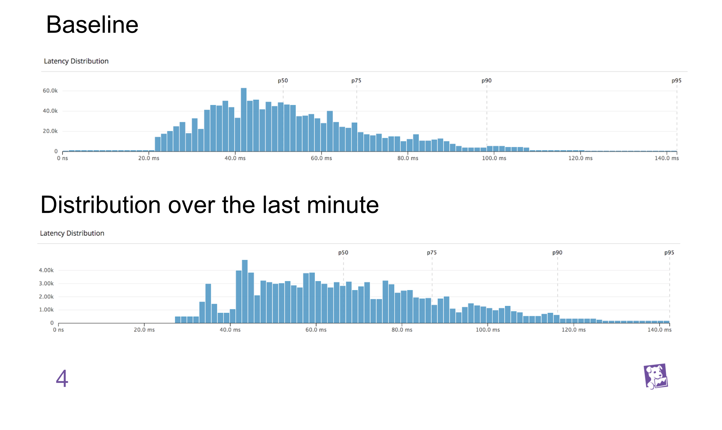
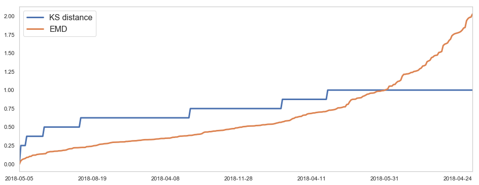
For example, is the current latency distribution anomalous?
Detailed review with Mathematics
Probability distribution
- $K$: State space (For instance, $K=\mathbf{R}$ or compact subset in $\mathbf R^d$)
$\mathcal F$: $\sigma$-algebra(field) on $K$
- $K\in \mathcal F$
- If $A\in \mathcal F$, then $A^c \in \mathcal F$
- closed under countable union
Probability measure $\mathbf P$ on $(K, \mathcal F$)
- set function $\mathbf P : \mathcal F \to \mathbf R^+$ with $\mathbf P(K)=1$ (non negativity, null empty set, countable additivity)
- Probability distribution can be regarded as probability space $(K,\mathcal F,\mathbf P)$
Example1(continuous)
- $K = \mathbf R^d$, $\mathcal F$ $=\mathcal B(\mathbf R^d)$, Borel sets
- For $A\in \mathcal F$,
where
$$ p(x)=\frac{1}{\sqrt{(2\pi)^d |\Sigma|}} \exp \left(-\frac{1}{2} (x-\mu)^T \Sigma^{-1}(x-\mu) \right), $$mean vector $\mu\in \mathbf R^d$, covariance matrix $\Sigma \in \mathbf R^{d\times d}$, and det$(\Sigma)=|\Sigma |$.
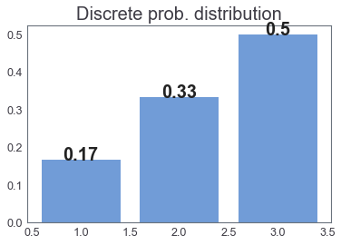
Example2(discrete)
- $K=\{ 1$$,2,3 \}$
- $\mathcal F=$ $\mathcal P(K)$, power set
Main Goal: Compare two distributions
Let $B$ and $T$ be $\color{red}{\bf{unknown}}$ 1-dimensional prob. distributions.
$K:=\mathbf R$, $\mathcal F:= \mathcal B(\mathbf R)$
$$ B=(\mathbf R,\mathcal F,\mathbf P), \,T=(\mathbf R,\mathcal F,\mathbf Q)\, \text{ two prob. spaces} $$Goal: Compare two samples drawn from $B$ and $T$
$$ B_N=\{ b_1, ..., b_N \}, \, b_i \text{ are ordered iid samples(observations) of } B $$$$ T_M=\{ t_1, ..., t_M \}, \, t_j \text{ are ordered iid samples(observations) of } T $$$b_i, t_j \in \mathbf R$.
Hypothesis
- $H_0 :=$ Both samples are drawn from the same distributions
- $H_a :=$ not $H_0$
Let us see single sample statistics
from scipy import stats
import scipy
import numpy as np
import seaborn as sns
import sys
import matplotlib.pyplot as plt
%matplotlib inline

print("Python version:", sys.version)
print("SciPy version:", scipy.__version__)
print("Numpy version:", np.__version__)
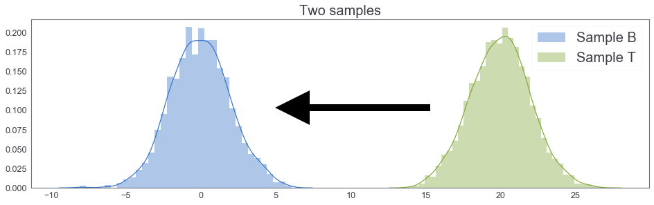
samples_plot()

mean of $B$ $<$ mean of $T$
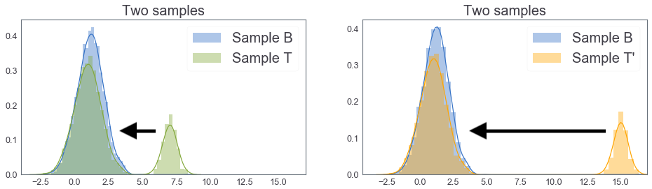
samples_plot2()

mean of $B$ $\sim$ mean of $T$ but $perc_{95}(T)< perc_{95}(B)$
samples_plot2()

$perc_{95}(T) \sim perc_{95}(B)$, but mean of $B$ $<$ mean of $T$
Simple sample statistics are not enough!
- Mean, median, TrMean, percentilie, standard deviation, skewness, IQR, ...
Need: statistical distance to measure difference between two samples
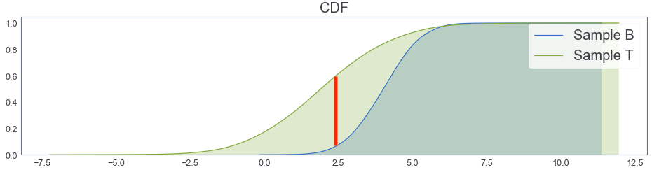
Focus on CDF!!
cum_plot()

KS distance(Kolmogorov-Smirnov) between 1-d two samples
- Non parametric method for comparing two samples
- Idea: comparing two empirical distribution functions(CDF)
 $$
KS(B, T):= \sup_{x\in \mathbf R} \left | F_B(x) - F_T(x) \right|
$$
$$
KS(B, T):= \sup_{x\in \mathbf R} \left | F_B(x) - F_T(x) \right|
$$
where
$$ F_B(x):= \frac{1}{N} \sum_{i=1}^N \chi_{(-\infty,x]}(b_i)= \frac{1}{N}\cdot \left(\# \, \text{of} \, b_i \leq x \right), $$and $\chi$ is an indicator function.
Decision rule of KS test
If
$$ KS(B,T) > \sqrt{ -\frac{\log(\alpha)}{2} } \sqrt{\frac{N+M}{NM}}, $$then the null hypothesis is rejected.
- $\alpha$: significant level(i.e. 0.05)
- $1-\alpha$: confidence coefficient
Or the p-value of $KS$ test $<$ $\alpha$, then $H_0$ is rejected.
KS distance is a metric.
Let $X$, $Y$, $Z$ be probability distraibutions.
$KS(X,Y)$ $\geq 0$
$KS(X,Y)$ $= 0$ if and only if $X=Y$
$KS(X,Y)$ $=$ $KS(Y,X)$
$KS(X,$ $Z)$ $\leq$ $KS(X$$,Y) +$$KS(Y$$,Z)$
KS distance in SciPy
scipy.stats.ks_2samp(data1, data2)
Computes the Kolmogorov-Smirnov statistic on 2 samples.
This is a two-sided test for the null hypothesis that 2 independent samples are drawn from the same continuous distribution.
- Parameters
- data1, data2: sequence of 1-D ndarrays, two arrays of sample observations assumed to be drawn from a continuous distribution, sample sizes can be different
- Returns
- statistic : float, KS statistic
- pvalue : float, two-tailed p-value
Example
from scipy import stats
n1 = 200
n2 = 300
For a different distribution, we can reject the null hypothesis since the pvalue is below 1%:
rvs1 = stats.norm.rvs(size=n1, loc=0., scale=1)
rvs2 = stats.norm.rvs(size=n2, loc=0.5, scale=1.5)
stats.ks_2samp(rvs1, rvs2)
(0.20833333333333337, 4.6674975515806989e-005)scipy.stats.ks_2samp(data1, data2)
data1 = np.sort(data1)
data2 = np.sort(data2)
n1 = data1.shape[0]
n2 = data2.shape[0]
data_all = np.concatenate([data1, data2])
cdf1 = np.searchsorted(data1, data_all, side='right') / (1.0 * n1)
cdf2 = np.searchsorted(data2, data_all, side='right') / (1.0 * n2)
d = np.max(np.absolute(cdf1 - cdf2))
# Note: d absolute not signed distance
en = np.sqrt(n1 * n2 / float(n1 + n2))
try:
    prob = distributions.kstwobign.sf((en + 0.12 + 0.11 / en) * d)
except:
    prob = 1.0

return Ks_2sampResult(d, prob)
cum_plot()

cum_plot(kde = False, bins = 1)

KS distance between two uniform distributions
3 samples: B, T, T'
two_cdfs()

Need: more appropriate distance
Joint Probability distribution with marginal $B$ and $T$
Continuous version
$$ \Gamma(B, T):= \left \{ \gamma: K \times K \longrightarrow \mathbf R^+\text{ s.t. }\int_K \gamma(x,y)dy = B(x)\text{ and }\int_K \gamma(x,y)dx = T(y) \right \} $$where $B(x)$ (resp. $T(y)$) is a density function of $B$(resp. $T$).
$\Gamma(B,T)$ is a set of pdf on $K\times K$ whose marginal dfs are $B$ and $T$.
Discrete version
$$ \Gamma(B, T):= \left \{ \gamma: K \times K \longrightarrow [0,1]\text{ s.t. }\sum_{y\in K} \gamma(x,y) = B(x)\text{ and }\sum_{x \in K} \gamma(x,y) = T(y) \right \} $$where $B(x)$ (resp. $T(y)$) is a probability mass function of $B$(resp. $T$).
$\Gamma(B,T)$ is a set of pmf on $K\times K$ whose marginal pmf are $B$ and $T$.
Earth mover's distance a.k.a. $1^{st}$ Wasserstein distance
(introduced by Leonid Vaseršteĭn(Russia))
$$\begin{align*} EMD(B,T) = W_1 (B,T) &= \inf_{\gamma \in \Gamma(B,T)} \int_{K\times K} |x-y| d\gamma(x,y) \quad \text{(continuous)}\\ & \\ &=\inf_{\gamma \in \Gamma(B,T)} \sum_{x,y} |x-y| \gamma(x,y) \quad \text{(discrete)} \end{align*} $$Remark
- $EMD(B,T) = \inf_{\gamma \in \Gamma(B,T)} E_{(x,y) \sim \gamma} \left [ |x-y| \right ]$
- $\gamma(x, y)$ can be seen as an amount of sand to move from $x \in B$ to $y \in T$
- Intuitively, $EMD$ is a minimum cost to move sand to another region(Optimal transport problem)
Another formulation $\color{red}{only}$ in case $K = \mathbf R$
Let $K = \mathbf R$. Then we have another formulation:
$$ EMD(B,T) = \int_{\mathbf R} |F_B(x) - F_T(x)| dx $$where $F_B$ is the CDF of $B$.
- Ref: On Wasserstein Two Sample Testing and Related Families of Nonparametric Tests
For your information, KS distance was the following:
$$ KS(B, T):= \sup_{x\in \mathbf R} \left | F_B(x) - F_T(x) \right| $$Remark
- $B$$=$ $\delta_s$ and $T$$=$ $\delta_t$, $s,t$ $\in$ $ \mathbf R$
$\quad \Rightarrow EMD(B, T)=|s-t|.$
- $B=N(\mu_1, C_1)$ and $T=N(\mu_2, C_2)$ on $\mathbf R^d$ where mean vectors $\mu_1, \mu_2 \in \mathbf R^d$, covariance matrices $C_1, C_2 \in \mathbf R^{d\times d}$.
$\quad \Rightarrow W_2(B, T)^2= \| \mu_1 - \mu_2\|^2 + tr(C_1 +C_2 -2 (C_2^{1/2} C_1 C_2^{1/2})^{1/2}).$
1st Wasserstein distance in SciPy
scipy.stats.wasserstein_distance(u_values, v_values, u_weights=None, v_weights=None)
Compute the first Wasserstein distance between two 1D distributions.
- Parameters
- u_values, v_values: array_like, Values observed in the (empirical) distribution.
- u_weights, v_weights: array_like, optional, Weight for each value. If unspecified, each value is assigned the same weight. u_weights (resp. v_weights) must have the same length as u_values (resp. v_values). If the weight sum differs from 1, it must still be positive and finite so that the weights can be normalized to sum to 1.
- Returns
- distance: float, The computed distance between the distributions.
two_cdfs2()
EMD between two uniform distributions
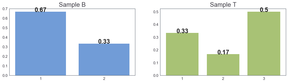
B = [1, 1, 2] # Sample B
T = [1, 1, 2, 3, 3, 3] # Sample T

print("EMD between B and T:", stats.wasserstein_distance(B,T))

v1, w1 = [1, 2], [2, 1] # Sample B
v2, w2 = [1, 2, 3], [2, 1, 3] # Sample T

print("EMD between B and T:", stats.wasserstein_distance(v1, v2, w1, w2))
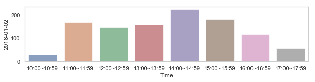
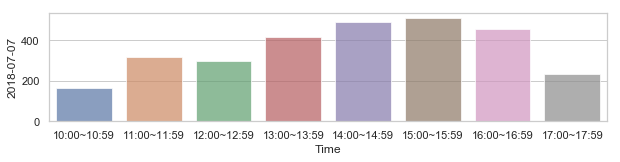
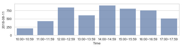
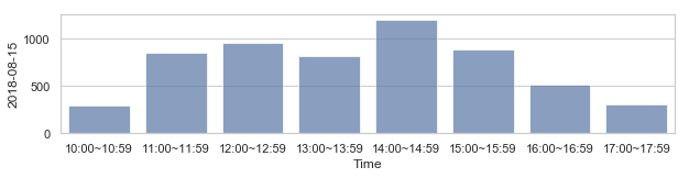
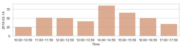
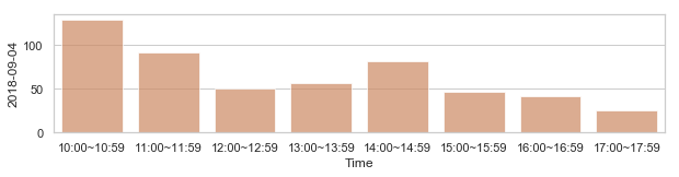

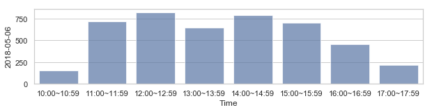
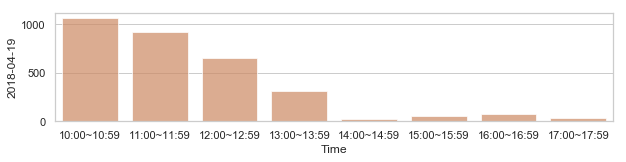
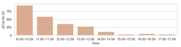
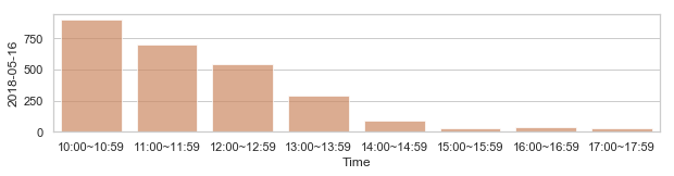
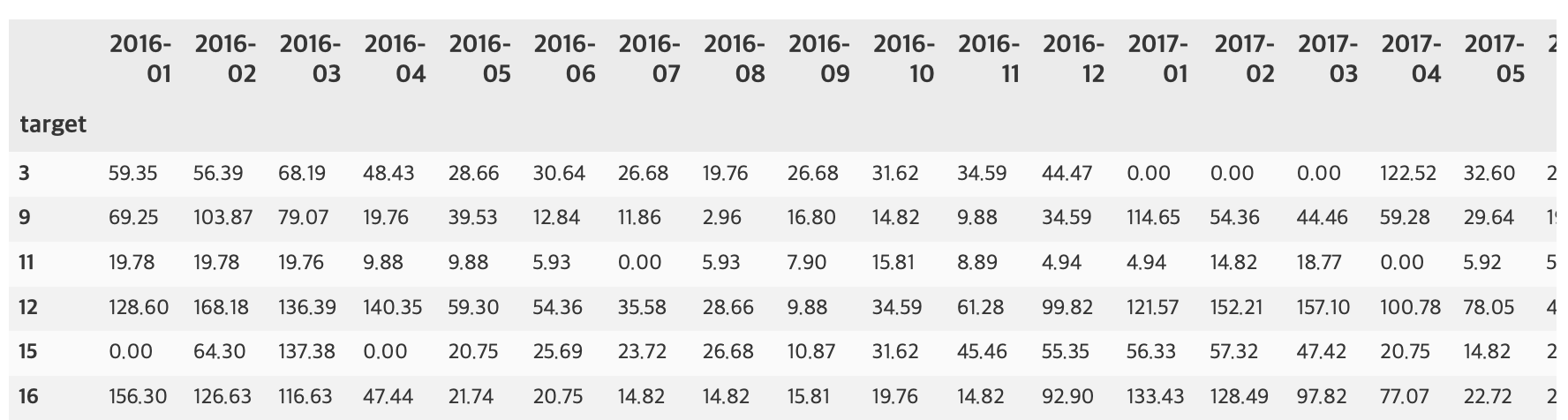
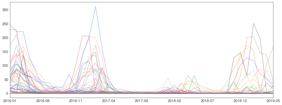
부산지역 582,184 세대별 도시가스 사용량
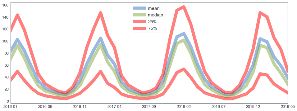
582,184 세대 평균과 유사한 패턴을 띄는 세대 top 50
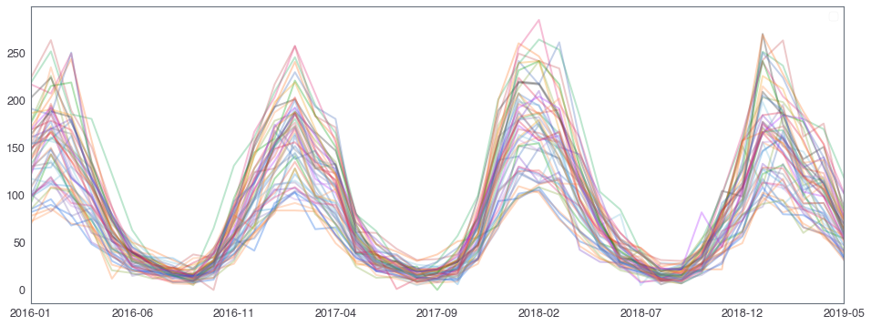
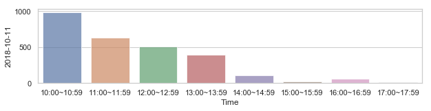
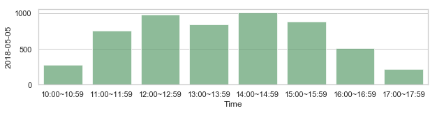
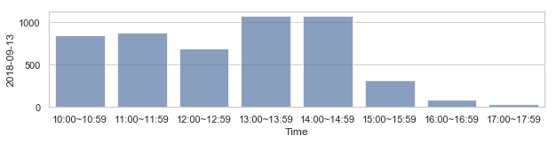
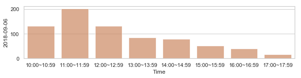
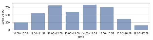
582,184 세대 평균과 다른 패턴을 띄는 세대 top 2000
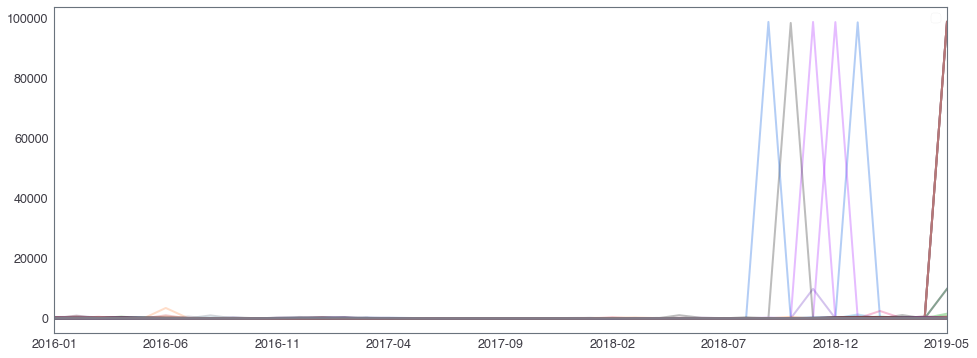
58,2184 세대 평균과 다른 패턴을 띄는 세대
Earth mover's distance with Linear programming
Treat each sample set $B$ corresponding to a “point” as a discrete probability distribution, so that each sample $x \in B$ has probability mass $p_x = 1 / |B|$. The distance between $B$ and $T$ is the optional solution to the following linear program.
Each $x \in B$ corresponds to a pile of dirt of height $p_x$, and each $y \in T$ corresponds to a hole of depth $p_y$. The cost of moving a unit of dirt from $x$ to $y$ is the Euclidean distance $d(x, y)$ between the points (or whatever hipster metric you want to use).
Let $\gamma(x, y)$ be a real variable corresponding to an amount of dirt to move from $x \in B$ to $y \in T$, with cost $d(x, y)$. Then the constraints are:
- Each $\gamma(x, y) \geq 0$, so dirt only moves from $x$ to $y$.
- Every pile $x \in B$ must vanish, i.e. for each fixed $x \in B$, $\sum_{y \in T} \gamma(x, y) = p_x$.
- Likewise, every hole $y \in T$ must be completely filled, i.e. $\sum_{x \in B} \gamma(x, y) = p_y$.
The objective is to minimize the cost of doing this: $\sum_{x, y \in B \times T} d(x, y) \gamma(x, y)$.
import math
import numpy as np
from collections import Counter
from collections import defaultdict
from ortools.linear_solver import pywraplp

def euclidean_distance_2(x, y):
    return math.sqrt(sum((a - b) ** 2 for (a, b) in zip(x, y)))

def euclidean_distance_1(x, y):
    return math.sqrt((x - y) ** 2 )

def earthmover_distance(p1, p2):

    if np.array(p1).shape[-1] == 2:
        euclidean_distance = euclidean_distance_2
    else:
        euclidean_distance = euclidean_distance_1
    '''
    Output the Earthmover distance between the two given points.
    '''
    dist1 = {x: count / len(p1) for (x, count) in Counter(p1).items()}
    dist2 = {x: count / len(p2) for (x, count) in Counter(p2).items()}

    if len(set(p2).difference(p1)) >0:
        for x in set(p2).difference(p1):
            dist1[x] = 0.

    if len(set(p1).difference(p2)) >0:
        for x in set(p1).difference(p2):
            dist2[x] = 0.


    solver = pywraplp.Solver("earthmover_distance",
                             pywraplp.Solver.GLOP_LINEAR_PROGRAMMING)

    variables = dict()

    dirt_leaving_constraints = defaultdict(lambda: 0)
    dirt_filling_constraints = defaultdict(lambda: 0)

    # the objective
    objective = solver.Objective()
    objective.SetMinimization()

    for (x, dirt_at_x) in dist1.items():
        for (y, capacity_of_y) in dist2.items():
            amount_to_move_x_y = solver.NumVar(0,
                             solver.infinity(), "z_{%s, %s}" % (x, y))
            variables[(x, y)] = amount_to_move_x_y
            dirt_leaving_constraints[x] += amount_to_move_x_y
            dirt_filling_constraints[y] += amount_to_move_x_y
            objective.SetCoefficient(amount_to_move_x_y,
                                     euclidean_distance(x, y))

    for x, linear_combination in dirt_leaving_constraints.items():
        solver.Add(linear_combination == dist1[x])

    for y, linear_combination in dirt_filling_constraints.items():
        solver.Add(linear_combination == dist2[y])

    status = solver.Solve()
    if status not in [solver.OPTIMAL, solver.FEASIBLE]:
        raise Exception("Unable to find feasible solution")

    for ((x, y), variable) in variables.items():
        if variable.solution_value() != 0:
            cost = euclidean_distance(x, y) * variable.solution_value()

    return objective.Value()
v1 = [1, 1, 2]

v2 = [1, 1, 2, 3, 3, 3]

print(earthmover_distance(v1, v2))
print(stats.wasserstein_distance(v1, v2))
print(earthmover_distance(rvs3[: : 3], rvs4[: : 3]))
# >>> 29 s ± 139 ms per loop (mean ± std. dev. of 7 runs, 1 loop each)

print(stats.wasserstein_distance(rvs3[: : 3], rvs4[: : 3]))
# >>> 424 µs ± 2.81 µs per loop (mean ± std. dev. of 7 runs, 1000 loops each)
Why Wasserstein distance is weak.
The learning a probability distribution of a data is very important for machine learning
- $\mathbf P_r$: target prob. measure(distribution)
- $\mathbf P_\theta$: prob. measure parametrized by $\theta$
Maximum Likelihood method
$$ \max \color{red}{\text{Likelihood}} \iff \min \color{red}{KL(\mathbf P_r | \mathbf P_\theta)} \iff \min\color{red}{\text{cross-entropy}} $$However, $KL$-divergence sometimes overshoot!
Relation between distances
Statistical distances
- total variation distance, $\delta(\mathbf P, \mathbf P_n)$
- KL-divergence, $KL(\mathbf P | \mathbf P_n)$
- Wasserstein distance, $W(\mathbf P, \mathbf P_n)$
Relation
- $\mathbf P$: fixed prob. measure on $(K, \mathcal F)$
- $(\mathbf P_n)_n$: seq. of prob. distributions on $(K, \mathcal F)$
Let $n\to \infty$, then $$ \delta(\mathbf P, \mathbf P_n) \to 0 \iff KL(\mathbf P | \mathbf P_n) \to 0 \iff KL(\mathbf P_n | \mathbf P) \to 0. \qquad (*) $$
Furthermore, $(*)$ with $n\to \infty$ implies
$$ W(\mathbf P, \mathbf P_n) \to 0. $$Finite signed measure space
Let $K\subset \mathbf R^d$ be a compact and $\mathcal F:= \mathcal B(K)$. Let $\mu$ be a finite signed measure on $(K, \mathcal F)$ (by Hahn decomposition, uniquely devided by finite measures $\mu_+, \mu_-$) and total variation norm
$$\begin{align*} \| \mu \|_{TV}:&= \sup_{A\in \mathcal F} |\mu(A)| + |\mu(A^c)|\\ &= \mu_+(K) + \mu_-(K) \end{align*}$$Let $$ \mathcal M := \left \{ \mu :\text{finite signed measure on }(K, \mathcal F) \right \}. $$
Then $\mathcal M$ is a Banach space w.r.t. $\| \mu \|_{TV}$.
$$ Prob(K):=\text{ all prob. measures on }(K, \mathcal F). $$Then $Prob(K)$ is a closed subspace of $\mathcal M$, complete itself.
For $\mu, \nu \in Prob(K)$, total variation distance defined by
$$ \delta(\mu, \nu):= \| \mu - \nu \|_{TV}= \sup_{A\in \mathcal F} |\mu(A) - \nu(A)| + |\mu(A^c)-\nu(A^c)| $$is a distance in $Prob(K)$.
Continuous function space on a compact set $K$ and its dual
Consider
$$ C(K):= \{ f: K \to \mathbf R, \text{ continuous} \} $$with norm $\| f\|_\infty := \max_{x\in K} |f(x)|$. Then $(C(K), \| \cdot \|_\infty)$ is a normed space. Define its dual
$$ C(K)^*:= \{ \phi: C(K) \to \mathbf R, \text{ linear and continuous} \} $$with dual norm $\| \phi \| := \sup_{f\in C(K), \, \|f \|_\infty\leq 1} |\phi(f)|$.
$\Rightarrow$ $(C(K)^*, \|\cdot \|)$ is another normed space.
Isometric immersion
$$ \Phi: (Prob(K), \delta) \longrightarrow (C(K)^* , \| \cdot \|) $$$$ \Phi(\mu)(f) = \int_K f d\mu, \quad\text{ for }\, f \in C(K), \, \mu\in Prob(K) $$Then $\Phi$ is an isometric immersion.
It means that $(Prob(K), \delta)$ can be as a subset of $(C(K)^*, \|\cdot \|)$ or total variation distance $\delta$ over $Prob(K)$ is exactly the norm distance over $C(K)^*$.
Dual space $C(K)^*$ has a weak$^*$ topology which is weaker than the strong topology induced by $\| \cdot \|$.
In the case of $Prob(K) (\subset C(K)^*)$, the strong topology is given by the total variation, but weak$^*$ topology is given by the Wasserstein distance.
Consider two probability measure $\mathbf P, \mathbf Q$ on $(K, \mathcal F)$.
1. Total variation distance
$$ \delta(\mathbf P, \mathbf Q):= \| \mathbf P - \mathbf Q \|_{TV} = \sup_{A\in \mathcal F} | \mathbf P(A) - \mathbf Q(A)| + |\mathbf P(A^c)-\mathbf Q(A^c)| $$2. $KL$-divergence(Kull back-Leibler)
$$ KL(\mathbf P | \mathbf Q) := \int_K \log \left (\frac{p(x)}{q(x)} \right) p(x) \mu (dx) $$where $\mathbf P$ and $\mathbf Q$ are absolutely continuous w.r.t. $\mu$ on $K$ $(A\in \mathcal F$ if $\mu(A) = 0 $, then $\mathbf P(A) = \mathbf Q(A) = 0)$.
3. Jensen-Shannon(JS) divergence
$$ JS(\mathbf P, \mathbf Q):= KL(\mathbf P | \mathbf M) + KL(\mathbf Q | \mathbf M) $$where $\mathbf M:= (\mathbf P + \mathbf Q)/2$.
4. EM distance, 1$^{st}$ Wasserstein distance
$$ \inf_{\gamma \in \Gamma(\mathbf P, \mathbf Q)} E_{(x,y)\sim \gamma} [|x-y|] $$Let $\mathbf P$ be a prob. measure on $K$ and $(\mathbf P_n)_n$ be a seq. of prob. measures on $K$.
1. The following statements are equivalent.
$$\begin{align*} & \delta(\mathbf P_n , \mathbf P) \to 0 \text{ as }n \to \infty.\\ & \qquad \qquad \qquad\qquad\qquad\qquad (*)\\ & JS(\mathbf P_n , \mathbf P) \to 0 \text{ as } n \to \infty. \end{align*}$$2. The following statements are equivalent.
$$\begin{align*} & W(\mathbf P_n , \mathbf P) \to 0 \text{ as }n \to \infty.\\ & \\ & \mathbf P_n \to \mathbf P\text{ converges in distribution for r.v. as }n \to \infty \end{align*}$$3. $KL(\mathbf P_n | \mathbf P) \to 0$ or $KL(\mathbf P | \mathbf P_n) \to 0$ as $n\to \infty$ implies $(*)$
4. 1. implies 2.
Reference
- On Wasserstein Two-Sample Testing and Related Families of Nonparametric Tests
- Concrete representation of abstract (m)-spaces (a characterization of the space of continuous functions)
- Optimal Transport
- Wasserstein GAN
- Earthmover Distance: https://jeremykun.com/tag/wasserstein-metric/