Anomaly Detection with Scikit learn
https://mjgim.io/slides/AD2020/Anomaly_detection.slides.html
Minjung Gim(mjgim@nims.re.kr) at NIMS
2020
Goal
- Overview of Anomaly detection
- Introduction of methods
- Classic algorithms provided by Scikit-learn
Anomaly detection: 이상 감지
- Task of discerning unusual samples in data
- Process of identifying unexpected observation or event in data
- (it is treated as an unsupervised learning problem)
Synonym of Anomaly
- Abnormal or anomalous observation, abnormality, outlier, novelty, etc.
What is anomalies?
- Actually, not easy to define and subjective
- Samples that do not fit to a general, well-defined and normal pattern
- Simply, few and different samples
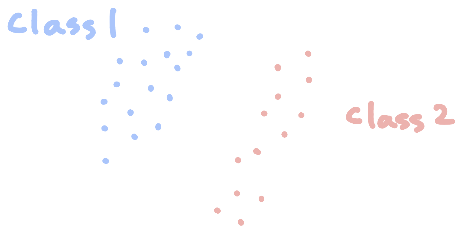
- In this lecture, we have only two labels(normal and abnormal)
Anomaly detection is complicated because:
- Anomalies are hard to define
- Inaccurate boundaries between the outlier and normal behavior
- Labeled data might be hard (or even impossible) to obtain
- Imbalanced data set
- Noise in the data which mimics real outliers and therefore makes is challenging to distinguish and remove them
Masking effect: the presence of another adjacent ones(colluder)
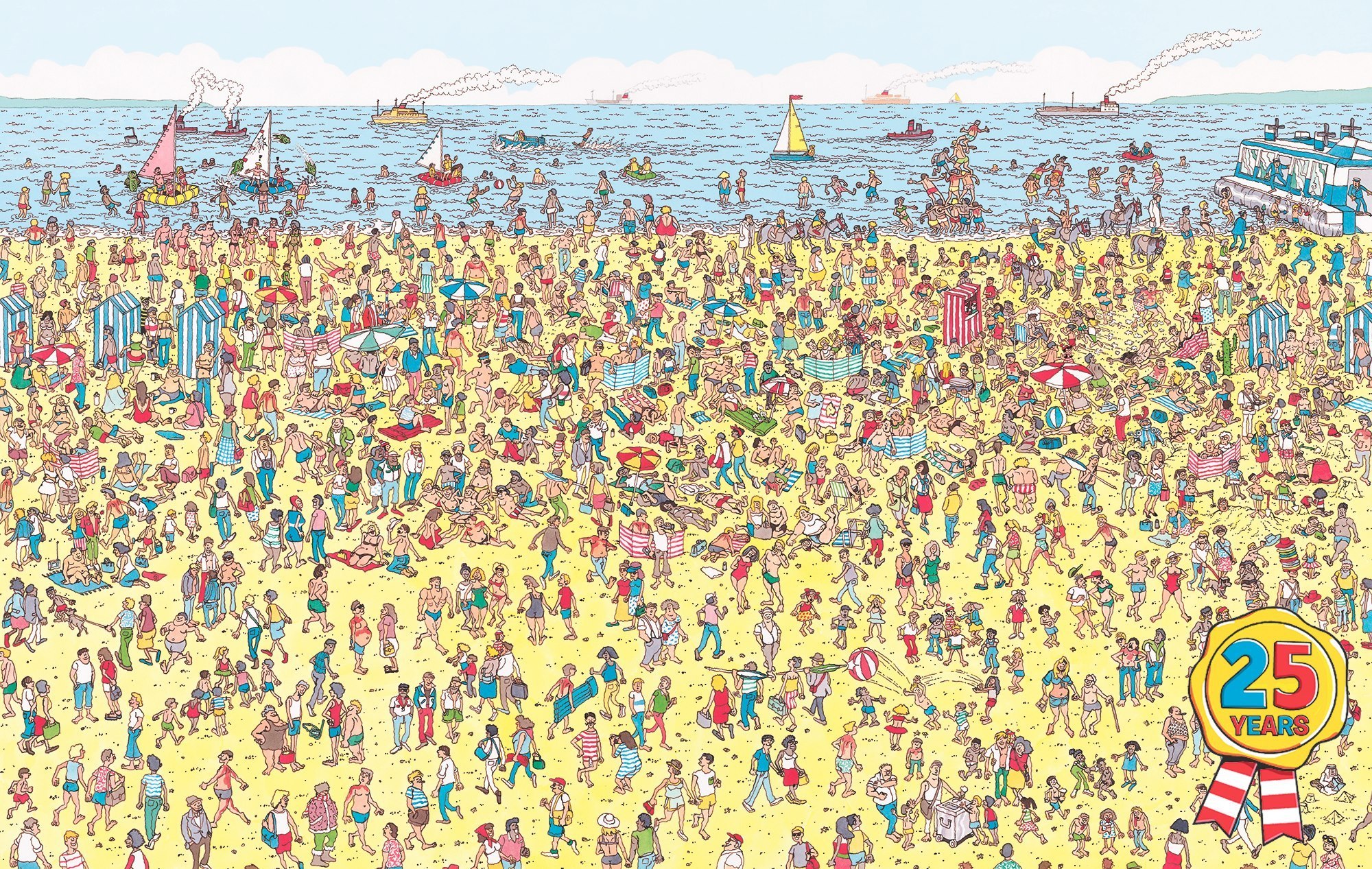 Image source: Where is Wally?
Type of anomalies
- Anomalies can be classified into three types:
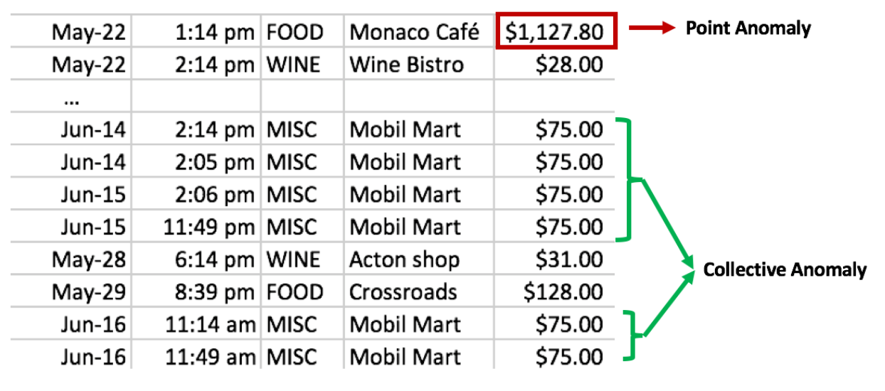
1. Point anomalies
- represent an irregularity or deviation that happens randomly and may have no particular interpretations
2. Contextual(conditional) anomalies
- identified by considering both contextual and behavioural features
3. Group(collective) anomalies
- each of the individual points in isolation appears as normal data instances while observed in a group exhibit unusual characteristics
Prior knowledge
- Anomaly detection can be divided by supervised, unsupervised and semi-supervised learning
1. Binary classification
- labeled sample consisting of both normal and anomalous examples
2. Highly imbalanced binary classification
- data set contains few anomalies
3. Outlier detection
- unlabeled sample that is contaminated with abnormal instances. An estimation for the expected ratio of anomalies is often known in advance.
4. One class classification(semi-supervised)
- samples only from a normal class of instances and the goal is to construct a classifier capable of detecting out-of-distribution abnormal instances
Scikit learn
Outlier detection
- The training data contains outlier that are far from the others
- Outlier detection estimators try to fit the regions where the training data is the most concentrated.
Novelty detection
- The training data is not polluted by outliers and we are interested in detecting whether a new observation is an outlier(called novelty)
- Assume that all observations in training data is normal
In novelty detection, there may be normal samples in the training data that are far from other points.
Application areas
not important
- Data logs and process logs
- Fraud detection and intrusion detection
- Security and surveillance
- Fake news and information, social networks
- Health case analysis and medical diagnosis
- Data sources of transactions
- Sensor networks and databases
- Data quality and data cleaning
- Time series monitoring and data streams
- Internet of things
Needs domain knowledge
Methods
not important
A. Statistical based approaches
- Parametric and non-parametric methods
- Data points are modeled using a well known stochastic distribution
- Robust covariance, Gaussian mixture model(GMM), Kernel density estimation(KDE)
B. Density based approaches
- Outlier can be found in a low-density region whereas inlier are assumed to appear in dense neighborhoods
- Consider the neighborhood of an object which is defined by a given radius
Methods'
not important
C. Distance based approaches
- Detect outliers by computing the distances between points
- A point, a far distance from its nearest neighbor is regarded as an outlier
- So not robust to scale variance
- Local Outlier Factor(LOF)
D. Clustering based approaches
- Use clustering methods to describe the behavior of the data
- Points in smaller size clusters are deemed as outliers
E. Reconstruction based or Deep approaches
Classifier(decision function) performance
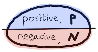
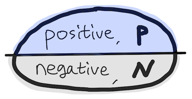
- Assume that we know the labels of test data $X$(essential)
- Evaluate a binary classifier(decision function) $$ h(x): X \longrightarrow \{ 0, 1\} $$
- WLOG, 1 means outlier(positive) and 0 label means inlier(negative)
- The best classifier satisfies that
and
$$ h(x) = 0 \text{, whenever } x \text{ is an inlier} $$Accuracy is not a good measure for assessing a classifier
- There are 9990 normal observations but only 10 anomalous observations
- Example
| Positive prediction | Negative prediction | total | |
|---|---|---|---|
| Outlier(positive) | 0 | 10 | 10 |
| Inlier(negative) | 0 | 9990 | 9990 |
| total | 0 | 10000 | 10000 |
- Baseline of Accuracy
where $N$: the number of negative observations and $P$: the number of positive observations
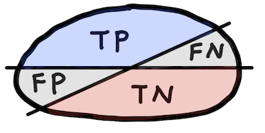
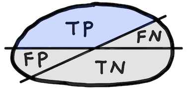
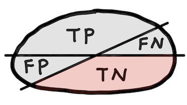
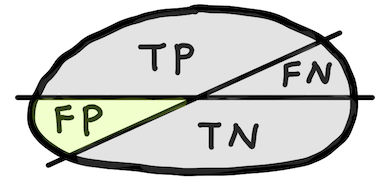
Confusion matrix
| Positive prediction | Negative prediction | |
|---|---|---|
| Observed positive | True positive (TP) | False negative (FN) |
| Observed negative | False positive (FP) | True negative (TN) |
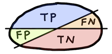
- TP: instance is positive and is classified as positive
- FN: instance is positive but is classified as negative
- TN: instance is negative and is classified as negative
- FP: instance is negative but is classified as positive
Accuracy
$$ \text{Accuracy}=\frac{\text{TP} + \text{TN}}{\text{P}+\text{N}} $$
|
|
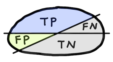
Sensitivity or Recall (True positive rate, TPR)
$$ \text{Sensitivity} = \frac{\text{TP}}{\text{P}} $$
|
|
Specificity (True negative rate, TNR)
$$ \text{Specificity} = \frac{\text{TN}}{\text{N}} $$
|

|
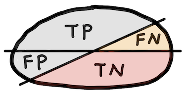
Precision (Positive predictive value, PPV)
$$ \text{Precision} = \frac{\text{TP}}{\text{TP+FP}} $$|
|
|
Negative predictive value, NPV
$$ \text{NPV} = \frac{\text{TN}}{\text{TN+FN}} $$|
|
|
False positive rate, FPR
$$ \text{FPR} = \frac{\text{FP}}{\text{N}} = 1-\text{TNR} $$
|
|
Evaluation metric
- Confusion matrix
| Positive prediction | Negative prediction | |
|---|---|---|
| Observed positive | True positive (TP) | False negative (FN) |
| Observed negative | False positive (FP) | True negative (TN) |
- Evaluation metric
| Prediction based | label based |
|---|---|
| Positive predictive value $ = \frac{TP}{TP + FP}$ | True positive rate $ = \frac{TP}{P}$ |
| Negative predictive value $ = \frac{TN}{TN+FN}$ | True negative rate $ = \frac{TN}{N}$ |
| False positive rate $ = \frac{FP}{N}$ | |
| Accuracy $=\frac{TP + TN}{P+N}$ |
Evaluation metric`
- Example
| Positive prediction | Negative prediction | total | |
|---|---|---|---|
| Outlier(positive) | 3 | 15 | 18 |
| Inlier(negative) | 2 | 80 | 82 |
| total | 5 | 95 | 100 |
- Evaluation metric
| Prediction based | label based |
|---|---|
| Positive predictive value $ = \qquad\qquad$ | True positive rate $ = \qquad\qquad$ |
| Negative predictive value $ =\qquad \qquad$ | True negative rate $ = \qquad\qquad$ |
| False positive rate $ = \qquad\qquad$ | |
| Accuracy $=\qquad\qquad$ |
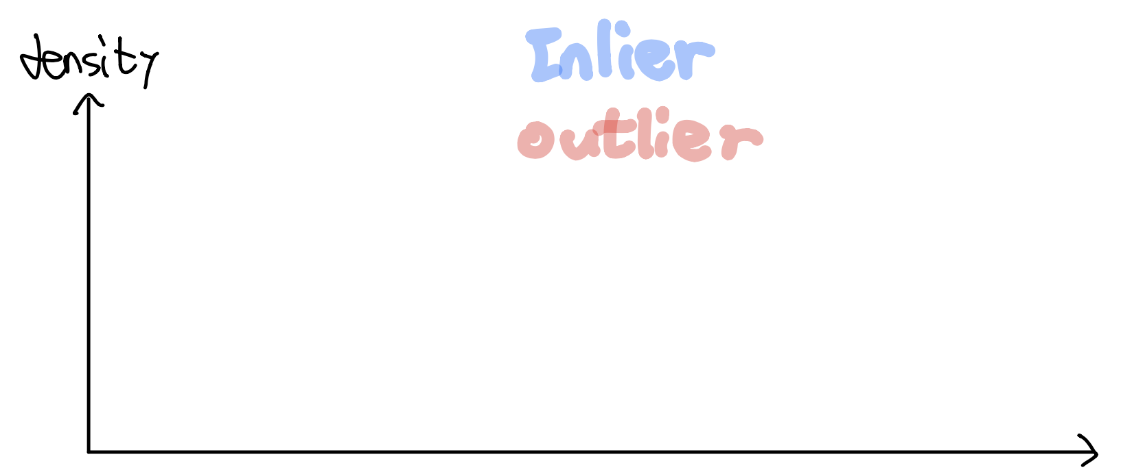
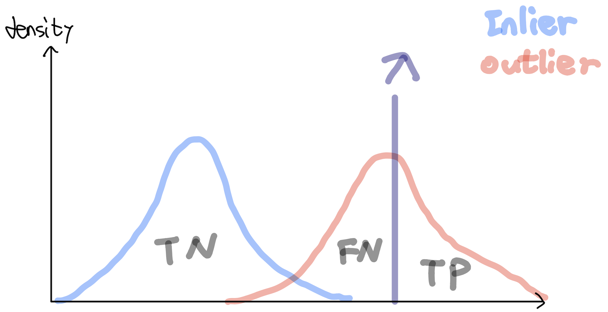
Scoring function(Anomaly score)
$$ s(x): X \longrightarrow \mathbb R $$Assume higher scores indicate that samples are more likely to be an outlier, e.g. $s(x)$ is indicated the estimated probability that the sample $x$ is an outlier.
Want: $s(X_{out})$ and $s(X_{in})$ are completely separated!
where $X_{out}$ is the collection of outliers in $X$ and $X_{in} = X\setminus X_{out}$ (we assumed that we know the labels of test data).
Once such a scoring function has been learned(obtained), a classifier can be constructed by threshold $\lambda \in \mathbb R$:
$$ h^\lambda (x):=\begin{cases} 1 &s(x) \geq \lambda \\ 0 &s(x)< \lambda \end{cases} $$Examples of scoring function
Examples of scoring function and evalution metric
Examples of scoring function
TPR and FPR
- True positive rate, TPR
- False positive rate, FPR
|
|
|
|
|
|
ROC(Receiver operating characteristic) curve
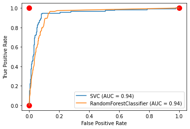
- 2 dim graph tp rate is plotted on the y-axis and fp rate is plotted on the x-axis
- Performance metric to measure the quality of the tradeoff of a scoring function $s(x)$
Tradeoffs between benefits(true positives rate) and cost(false positives or false alarm rate)
Classifier $h^\lambda(x)$ is determined by threshold $\lambda$ so one point in ROC graph is obtained by $\lambda$
Simply, for a scoring function $s(x)$
Several important points in ROC space
- $(0,0)$: the strategy of never issuing a positive classification; such a classifier commits no false
- $(0,1)$: perfect classification
- $(1,1)$: unconditionally issuing positive classifications
Random performance
- If it guesses the positive class $t\%$ of time, it can be expected to get $t\%$ of the positives correct but its false positive rate will be $t\%$ as well $(o\leq t \leq 100)$, yielding $(t,t)$ in ROC space
- The diagonal line $y=x$ represents the strategy of randomly guessing a class
- A classifier below the diagonal may be said to have useful information but it is applying the information incorrectly
Analysis of ROC space
- Informally, points to the northwest is better than others(tp rate is higher and fp rate is lower)
- Low fp rate mat be thought of as "conservative"; they make positive classifications only with strong evidence so they make few false positive errors(low true positive rates)
- High fp rate may be thought of as "liberal"; they make positive classifications with weak evidence so they classify nearly all positives correctly(high false positive rates)
AUROC
- Area under the ROC curve(AUROC) is a single scalar value representing expected performance
- Baseline of AUROC $= 0.5$, the area under line $y=x$
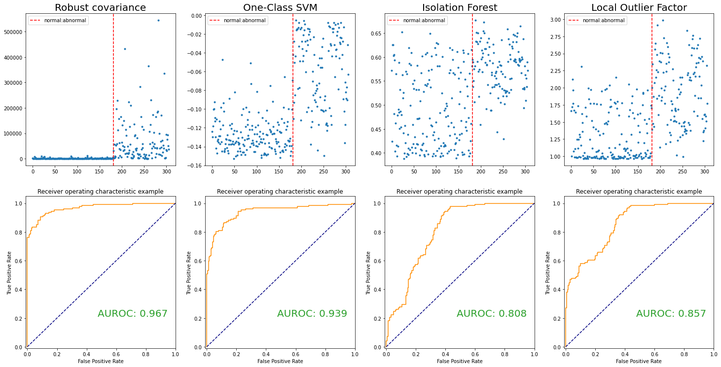
Robust Covariance(Minimum covariance determinant)
- Statistical based approach(parametric)
- (Assumption) Observations are sampled from an elliptically symmetric unimodal distribution(e.g. multivariate normal distribution)
- In other words, density function $f(\mathbf x)$, $\mathbf x\in\mathbb R^p$ can be written by
- where $d(\mathbf x, \mu, \Sigma) = \sqrt{(\mathbf x- \mu)^t \Sigma^{-1} (\mathbf x- \mu)}$ and a strictly decreasing real function $g$
Unknown parameters: location $\mu \in \mathbb R^p$ and scatter positive definite $p\times p$ matrix $\Sigma$
For instance, density function of the multivariate normal distribution
- i.e. $g(t)= \frac{1}{\sqrt{(2\pi)^p}} \exp(-\frac{t}{2})$
- Statistical distance $d(\cdot, \mu, \Sigma)$ represents how far away $\mathbf x$ is from the location $ \mu$ relative to scatter $\Sigma$
Aim to find $ \mu$, $\Sigma$ s.t. statistical distance is useful to detect outlier
Humble approach
- Using whole observations, compute location $\mu$ and scatter $\Sigma$ as:
and $$ \Sigma:=cov(X):= \frac{1}{N} \sum_{i=1}^N (\mathbf x_i - \bar{\mathbf x})(\mathbf x_i - \bar {\mathbf x})^t, \text{ (sample covariance)} $$
- In this case, the statistical distance is called Mahalanobis distance(MD)
- Because of Masking effect, not a good choice
Idea
- We need reliable estimators that can resist outliers when they occur. i.e. we need the ellipse that is smaller and only encloses the regular points.
- Try to remove masking effect, noise or outlier to yield a "pure" subset
- Idea is to find some (representitive) observations whose empirical covariance has the smallest determinant
Minimum covariance determinant
- Find $h$(fixed number) observations s.t. its determinant of covariance matrix is as samll as possilbe
- The larger $|\Sigma|$, the more dispersed
- Robust distance(RD) is defined by
- $\hat{\mu}_{MCD}$: MCD estimate of location (from $h$ observations)
$\hat{\Sigma}_{MCD}$: MCD covariance estimate (from $h$ observations)
Generally, ${N}\choose{h}$ is too many, so we need something...
Theorem(key)
Consider a data set $X:=\{ \mathbf x_1, ... ,\mathbf x_N \}$ of $p$-variate observations. Let $H_1 \subset \{1,...,N\}$ with $|H_1|=h$ and put
$$ T_1:= \frac{1}{h} \sum_{i\in H_1} \mathbf x_i, \quad S_1:= \frac{1}{h} \sum_{i\in H_1} (\mathbf x_i - T_1)(\mathbf x_i- T_1)^t. $$If $\det (S_1) \neq 0$, then define the relative distances
$$ d_1(i):= \sqrt{(\mathbf x_i - T_1)^t S_1^{-1}(\mathbf x_i- T_1)}, \text{ for } i=1,...,N. $$Sort these $N$ distances from the smallest $d_1(i_1)\leq d_1(i_2)\leq \cdots \leq d_1(i_N)$, then we obtain the ordered tuple $(i_1, i_2, ...,i_N)$(which is some permutaion of $(1,2,...,N)$). Let $H_2:=\{i_1,...,i_h\}$ and compute $T_2$ and $S_2$ based on $H_2$. Then
$$ \det(S_2) \leq \det(S_1) $$with equality if and only if $T_2=T_1$ and $S_2=S_1$.
Idea
Proof of Theorem
Proof. Assume that $det(S_2)>0$, otherwise the result is already satisfied. We can thus compute $d_2(i)=d_{(T_2, S_2)}(i)$ for all $i=1,...,N$. Using $|H_2|=h$ and the definition of $(T_2, S_2)$ we find
$$\begin{align*} \frac{1}{hp}\sum_{i\in H_2}d_2^2(i) &= \frac{1}{hp} tr \sum_{i\in H_2}(\mathbf x_i -T_2) S_2^{-1}(\mathbf x_i - T_2)^t \\ \tag{A.1} &=\frac{1}{hp} tr \sum_{i\in H_2}S_2^{-1}(\mathbf x_i -T_2) (\mathbf x_i - T_2)^t \label{A.1} \end{align*}$$Moreover, put
$$\begin{equation*} \tag{A.2} \lambda:= \frac{1}{hp} \sum_{i\in H_2} d_1^2(i) = \frac{1}{hp} \sum_{k=1}^h d_1^2(i_k)\leq \frac{1}{hp} \sum_{j\in H_1} d_1^2(j) =1, \label{A.2} \end{equation*}$$where $\lambda>0$ because otherwise $\det(S_1)=0$. Combining (\ref{A.1}) and (\ref{A.2}) yields
$$ \frac{1}{hp} \sum_{i\in H_2} d^2_{(T_1,\lambda S_1)}(i) = \frac{1}{hp} \sum_{i\in H_2}(\mathbf x_i -T_1)^t \frac{1}{\lambda}S_1^{-1}(\mathbf x_i - T_1) = \frac{1}{\lambda hp} \sum_{i\in H_2}d_1^2(i) =\frac{\lambda}{\lambda}=1. $$Proof of Theorem`
Grubel(1988) proved that $(T_2, S_2)$ is the unique minimizer of $\det(S)$ among all $(T,S)$ for which $\frac{1}{hp}\sum_{i\in H_2} d^2_{(T,S)}(i) = 1$. This implies that $\det(S_2)\leq det(\lambda S_1)$. On theother hand it follows from the inequality (\ref{A.2}) that $\det(\lambda S_1)\leq \det(S_1)$, hence
$$\begin{equation*} \tag{A.3} \det(S_2)\leq \det(\lambda S_1)\leq \det(S_1) \label{A.3} \end{equation*}$$Moreover, note that $\det(S_2)=\det(S_1)$ if and only if both inequalities in (\ref{A.3}) are equalities. For the first we know from Grubel's result that $\det(S_2)=\det(\lambda S_1)$ if and only if $(T_2, S_1)= (T_1,\lambda S_1)$. For the second, $\det(\lambda S_1) = \det(S_1)$ if and only if $\lambda = 1$, i.e. $S_1 = \lambda S_1$. Combining both tields $(T_2, S_2) = (T_1, S_1)$.
Method
- Fix $h$ s.t. $[(N+p+1)/2] \leq h \leq N$ and $h>p$
- Given the $h$-subset $H_{old}$ and its $(T_{old}, S_{old})$
- Compute $d_{old}(i)$ for $i=1,...,N$ and sort these distances which yields a permutation $\pi$ for which
- Let
- Compute
Tutorial
One class SVM(support vector machine)
- One class SVM is a variant of SVM(support vector machine)
- We have to understand SVM and kernel method(
however not easy)!
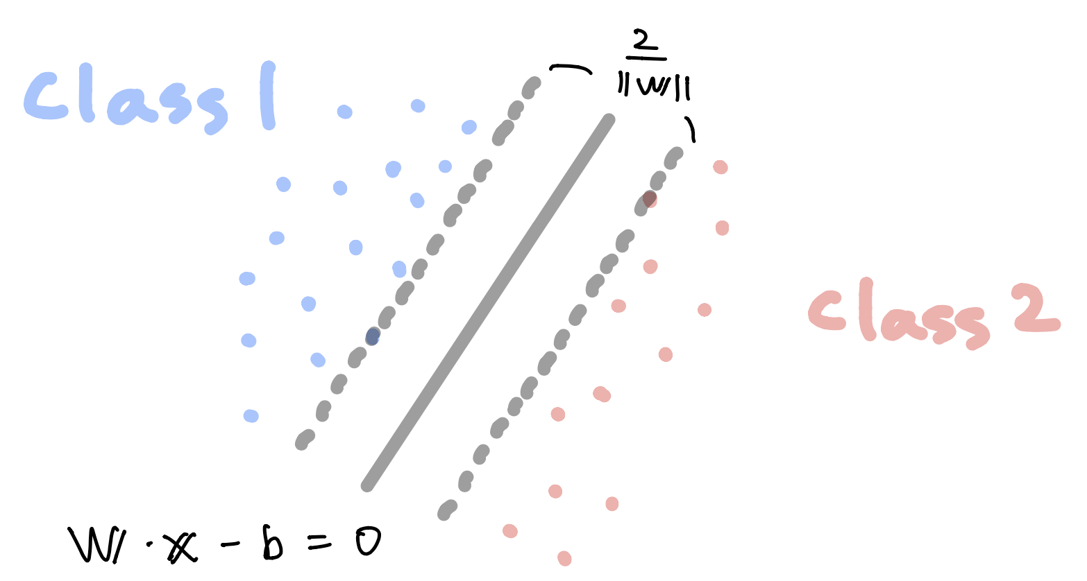
Linear SVM(simplest)
- Data matrix $X$, collection of $\mathbf x_i \in \mathbb R^p$ and its label $y_i= 1$ or $-1$
- SVM is a supervised learning method for classification(non-probabilistic binary linear classifier)
- Aim to find a $(p-1)$-hyperplane to separate two classes
Hard margin
- When $\mathbf x$ is on or above this boundary with label 1,
- When $\mathbf x$ is on or below this boundary with label -1,
Hard margin`
- Maximize $\frac{2}{\| \mathbf w \|}$ (i.e. minimize $\| \mathbf w \|$) with the following constraint
and
$$ \mathbf w \cdot \mathbf x_i - b \leq -1, \quad \text{ if } y_i =-1 $$- Rewrite
Soft margin
- Hinge loss
- $\lambda$: role of trade-off between margin size and ensuring that $\mathbf x_i$ lie on the correct side of the margin
- High $\lambda$ ~ underfitting (maximize margin)
- Low $\lambda$ ~ overfitting
Primal problem
- Note that $\zeta_i:= \max(0, 1- y_i(\mathbf w \cdot \mathbf x_i - b))$ is the smallest nonnegative number $t\geq 0$ satisfying
- So rewrite hinge loss as a quadratic optimization
Dual problem
- By solving for the Lagrangian dual of primal problem, we obtain the simplified problem
- Here the variables $c_i$ are defined such that
Nonlinear SVM
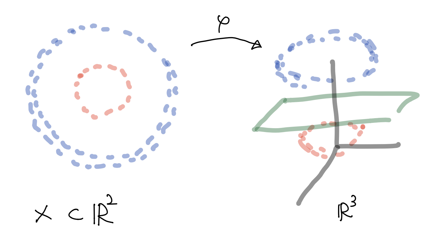
- Generally, data is not linearly separable
- Original maximum margin hyperplane classifier(1963)
Kernel method(1992)
For instance,
Nonlinear SVM`
- Feature map $\varphi: X \longrightarrow \cal F \subset \mathbb R^3$ given by(mapping the 2-dim data set to 3-dim feature space $\cal F$)
- Linear SVM classifier in this feature space $\cal F$
- Hyperplane in feature space $\cal F \subset \mathbb R^3$ can be determined by $\mathbf w=(w_1, w_2, w_3)$ and $b\in \mathbb R$ and expressed as
- This is nonlinear in $\mathbb R^2$
- But this is linear in feature space $\cal F$ (in $\mathbb R^3$)
Feature mapping(Kernel method)
- Feature map $\varphi: X \longrightarrow \cal F \subset \mathbb R^s$
- Find a maximal(soft) margin hyperplane in feature space $\cal F$
- Hinge loss(because we know the information of $\varphi$)
- Here $\mathbf w \in \mathbb R^s$ and $\mathbf w \cdot \varphi(\mathbf x_i)$ is an inner product in $\mathbb R^s$
Primal problem for feature mapped space
- So rewrite hinge loss as a quadratic optimization
Dual problem for feature mapped space
- By solving for the Lagrangian dual of primal problem, we obtain the simplified problem
- Here the variables $c_i$ are defined such that
Feature mapping(Kernel method)`
- Using feature map and finding hyperplane in feature space seems to be intuitive and easy
However, we have some problems:
- Unknown distribution of observations
Choice of feature map, e.g. random mapping $ \varphi: \mathbb R^2 \longrightarrow \mathbb R^\infty$
$$ \varphi(x_1, x_2):=(\sin(x_2), \exp(x_1+x_2), x_2, x_1^{\tan(x_2)},...) $$
Generally, dim of feature space may be high
- Lots of computation
Kernel method(Feature mapping)
- Feature mapping can be considered as a replacement of inner product by kernel function e.g.
- Question: Can not we say that(implicit) let
- there might exist a map $\varphi$ s.t. $k(\mathbf x, \mathbf y) = \varphi(\mathbf x)\cdot \varphi(\mathbf y)$ and feature space $\cal F$?
- Idea: Choose a nice kernel function $k$ rather than an ugly feature mapping(explicit)
- Only need to know $\varphi(\mathbf x_i)$, $\forall i =1,...,N$ not explicit $\varphi$
Kernel method(Feature mapping)`
Finite set
- $X = \{\mathbf x_1, ... , \mathbf x_N \}$, $\mathbf x_i \in \mathbb R^p$, $k:X \times X \longrightarrow [0, \infty)$, positive semi definite kernel
- Then we can construct a feature space $\cal F$ and feature map $\varphi$
- Let $G$ be a $N\times N$ matrix with $G_{ij}:=k(\mathbf x_i, \mathbf x_j)$ (can be calculated). Then $G$ is symmetric PSD so
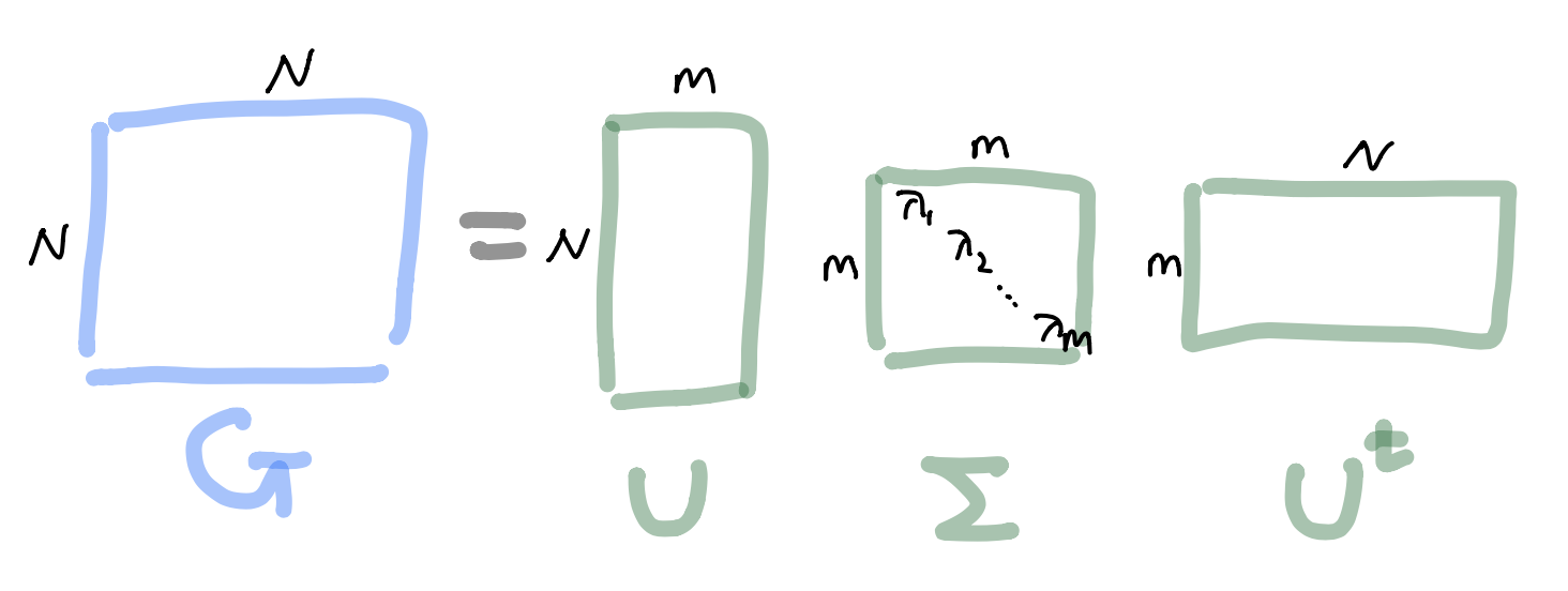
Kernel method(Feature mapping)``
Finite set
- Let $\varphi(\mathbf x_i):=\Sigma^{1/2} \mathbf u_i \in \mathbb R^m$, $i=1,...,N$
- Then such $\varphi(\mathbf x_i)$ leads to the Gram matrix $G$ because
Summary
- Given a psd kernel $k: X \times X \longrightarrow [0, \infty)$ and finite data set $X = \{\mathbf x_1, ... , \mathbf x_N \}$, $\mathbf x_i \in \mathbb R^p$
- Then we can construct a feature map $\varphi:X \longrightarrow \cal F$ and a feature space $\cal F = span \{ \varphi(\mathbf x_i) : \mathbf x_i \in$ $X \}$
- We can find a maximal margin hyperplane in $\cal F$, i.e. $\mathbf w \in \cal F$
Kernel trick
Dual problem
- By solving for the Lagrangian dual of primal problem, we obtain the simplified problem
- Here the variables $c_i$ are defined such that
- We may not know the explicit formula of $\varphi$. But for a new sample $\mathbf x$, we know that
One class SVM(2001)
- Finds a maximum (soft) margin hyperplane in feature space that best separates the mapped data from the origin
- Data matrix $X = \{\mathbf x_1, ... , \mathbf x_N \}$, $\mathbf x_i \in \mathbb R^p$
- OC-SVM solves the following primal problem(by quadratic programing)
- By Lagrangian dual of primal problem,
- $\mathbf w \cdot \varphi(\mathbf x) < \rho$ is deemed to be anomalous
Tutorial
Thank you for your attention!
with Datasaurus